How to p-hack (and avoid p-hacking) in ERP research

Luck, S. J., & Gaspelin, N. (2017). How to Get Statistically Significant Effects in Any ERP Experiment (and Why You Shouldn’t)Psychophysiology, 54, 146-157.

How to get a significant effect.jpg

In this article, we show how ridiculously easy it is to find significant effects in ERP experiments by using the observed data to guide the selection of time windows and electrode sites. We also show that including multiple factors in your ANOVAs can dramatically increase the rate of false positives (Type I errors). We provide some suggestions for methods to avoid inflating the Type I error rate.

This paper was part of a special issue of Psychophysiology on Reproducibility edited by Emily Kappenman and Andreas Keil.

An old-school approach to science: "You've got to get yourself a phenomenon"

Given all the questions that have been raised about the reproducibility of scientific findings and the appropriateness of various statistical approaches, it would be easy to get the idea that science is impossible and we haven't learned a single thing about the mind and brain. But that's simply preposterous.  We've learned an amazing amount over the years.

In a previous blog post (and follow-up), I mentioned my graduate mentor's approach, which emphasized self-replication. In this post, I go back to my intellectual grandfather, Bob Galambos, whose discoveries you learned about as a child even if you didn't learn his name. I hope you find his advice useful. It's impractical in some areas of science, but it's what a lot of cognitive psychologists have done for decades and still do today (even though you can't easily tell from their journal articles).  I previously wrote about this in the second edition of An Introduction to the Event-Related Potential Technique, and the following is an excerpt. I am "recycling" this previous text because the relevance of this story goes way beyond ERP research.


Galambos.jpg

My graduate school mentor was Steve Hillyard, who inherited his lab from his own graduate school mentor, Bob Galambos (shown in the photo).  Dr. G (as we often called him) was still quite active after he retired.  He often came to our weekly lab meetings, and I had the opportunity to work on an experiment with him.  He was an amazing scientist who made really fundamental contributions to neuroscience.  For example, when he was a graduate student, he and fellow graduate student Donald Griffin provided the first convincing evidence that bats use echolocation to navigate.  He was also the first person to recognize that glia are not just passive support cells (and this recognition essentially cost him his job at the time).  You can read the details of his interesting life in his autobiography and in his NY Times obituary.

Bob was always a font of wisdom.  My favorite quote from him is this: “You’ve got to get yourself a phenomenon” (he pronounced phenomenon in a slightly funny way, like “pheeeenahmenahn”).  This short statement basically means that you need to start a program of research with a robust experimental effect that you can reliably measure.  Once you’ve figured out the instrumentation, experimental design, and analytic strategy that allows you to reliably measure the effect, then you can start using it to answer interesting scientific questions.  You can’t really answer any interesting questions about the mind or brain unless you have a “phenomenon” that provides an index of the process of interest.  And unless you can figure out how to record this phenomenon in a robust and reliable manner, you will have a hard time making real progress.  So, you need to find a nice phenomenon (like a new ERP component) and figure out the best ways to see that phenomenon clearly and reliably.  Then you will be ready to do some real science!


Why I've lost faith in p values, part 2

In a previous post, I gave some examples showing that null hypothesis statistical testing (NHST) doesn’t actually tell us what we want to know.  In practice, we want to know the probability that we are making a mistake when we conclude that an effect is present (i.e., we want to know the probability of a Type I error in the cases where p < .05).  A genetics paper calls this the False Positive Report Probability (FPRP)

However, when we use NHST, we instead know the probability that we will get a Type I error when the null hypothesis is true. In other words, when the null hypothesis is true, we have a 5% chance of finding p < .05.  But this 5% rate of false positives occurs only when the null hypothesis is actually true.  We don’t usually know that the null hypothesis is true, and if we knew it, we wouldn't bother doing the experiment and we wouldn’t need statistics.

In reality, we want to know the false positive rate (Type I error rate) in a mixture of experiments in which the null is sometimes true and sometimes false.  In other words, we want to know how often the null is true when p < .05.  In one of the examples shown in the previous post, this probability (FPRP) was about 9%, and in another it was 47%.  These examples differed in terms of statistical power (i.e., the probability that a real effect will be significant) and the probability that the alternative hypothesis is true [p(H1)].

The table below (Table 2 from the original post) shows the example with a 47% false positive rate.  In this example, we take a set of 1000 experiments in which the alternative hypothesis is true in only 10% of experiments and the statistical power is 0.5. The box in yellow shows the False Positive Report Probability (FPRP).  This is the probability that, in the set of experiments where we get a significant effect (p < .05), the null hypothesis is actually true.  In this example, we have a 47% FPRP.  In other words, nearly half of our “significant” effects are completely bogus.

Why I lost faith in p values-2.jpeg

The point of this example is not that any individual researcher actually has a 47% false positive rate.  The point is that NHST doesn’t actually guarantee that our false positive rate is 5% (even when we assume there is no p-hacking, etc.).  The actual false positive rate is unknown in real research, and it might be quite high for some types of studies.  As a result, it is difficult to see why we should ever care about p values or use NHST.

In this follow-up post, I’d like to address some comments/questions I’ve gotten over social media and from the grad students and postdocs in my lab.  I hope this clarifies some key aspects of the previous post.  Here I will focus on 4 issues:

  1. What happens with other combinations of statistical power and p(H1)? Can we solve this problem by increasing our statistical power?

  2. Why use examples with 1000 experiments?

  3. What happens when power and p(H1) vary across experiments?

  4. What should we do about this problem?

If you don’t have time to read the whole blog, here are four take-home messages:

  • Even when power is high, the false positive rate is still very high when H1 is unlikely to be true. We can't "power our way" out of this problem.

  • However, when power is high (e.g., .9) and the hypothesis being tested is reasonably plausible, the actual rate of false positives is around 5%, so NHST may be reasonable in this situation

  • In most studies, we’re either not in this situation or we don’t know whether we’re in this situation, so NHST is still problematic in practice

  • The more surprising an effect, the more important it is to replicate

1. What happens with other combinations of statistical power and p(H1)? Can we solve this problem by increasing our statistical power?

My grad students and postdocs wanted to see the false positive rate for a broader set of conditions, so I made a little Excel spreadsheet (which you can download here).  This spreadsheet can calculate the false positive rate (FPRP) for any combination of statistical power and p(H1).  This spreadsheet also produces the following graph, which shows 100 different combinations of these two factors.

Why I lost faith in p values-3.jpg

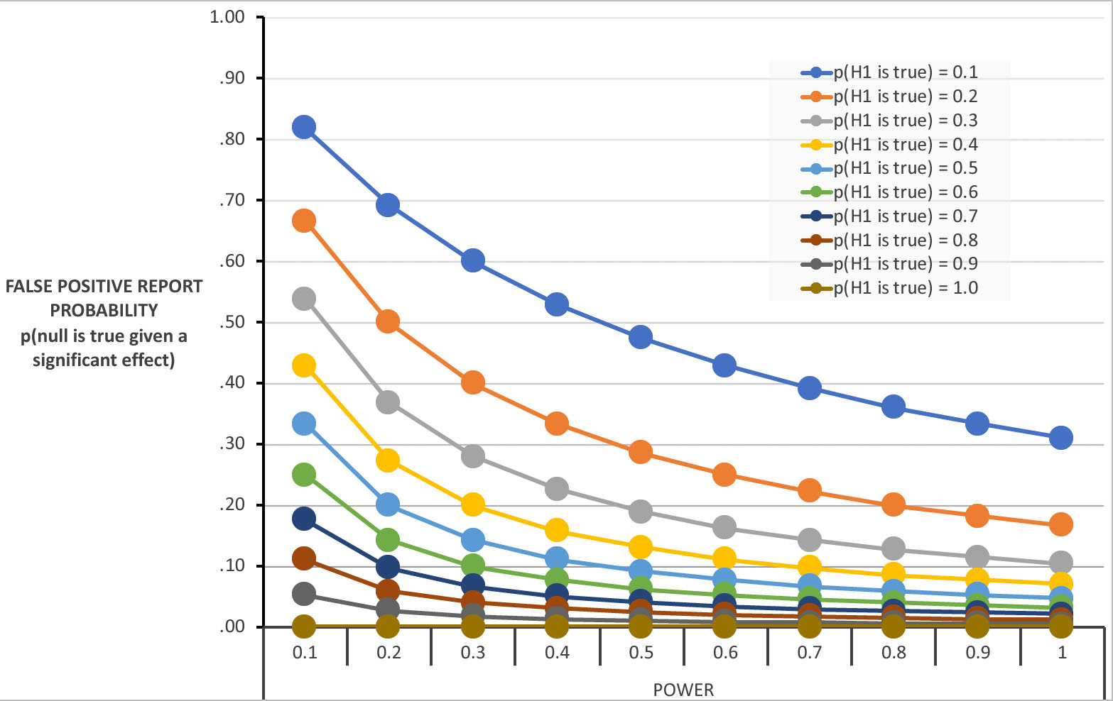
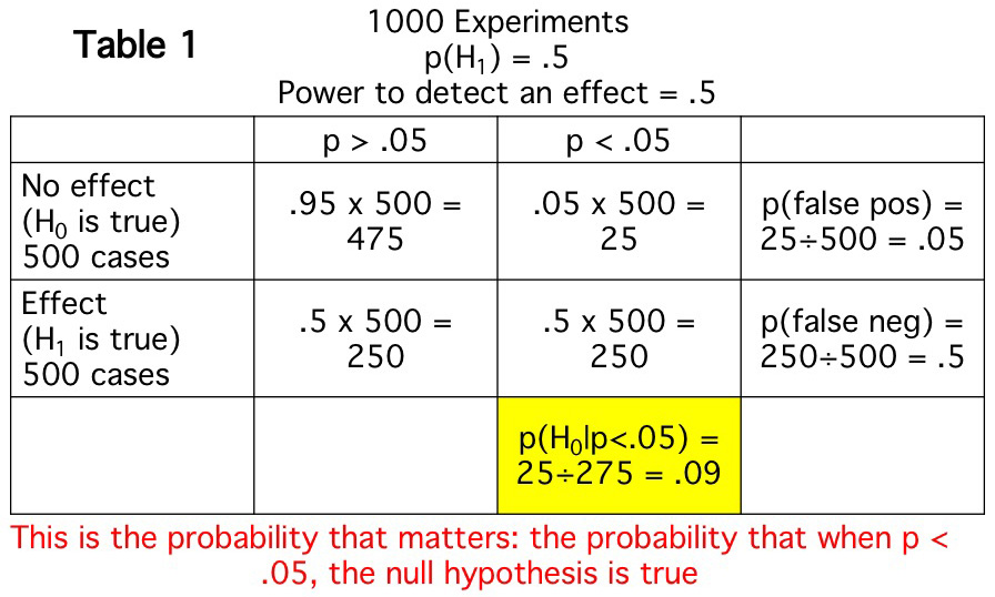
This figure shows the probability that you will falsely reject the null hypothesis (make a Type I error) given that you find a significant effect (p < .05) for a given combination of statistical power and likelihood that the alternative hypothesis is true.  For example, if you look at the point where power = .5 and p(H1) = .1, you will see that the probability is .47.  This is the example shown in the table above.  Several interesting questions can be answered by looking at the pattern of false positive rates in this figure.

Can we solve this problem by increasing our statistical power? Take a look at the cases at the far right of the figure, where power = 1.  Because power = 1, you have a 100% chance of finding a significant result if H1 is actually true.  But even with 100% power, you have a fairly high chance of a Type I error if p(H1) is low.  For example, if some of your experiments test really risky hypotheses, in which p(H1) is only 10%, you will have a false positive rate of over 30% in these experiments even if you have incredibly high power (e.g., because you have 1,000,000 participants in your study).  The Type I error rate declines as power increases, so more power is a good thing.  But we can’t “power our way out of this problem” when the probability of H1 is low.

Is the FPRP ever <= .05? The figure shows that we do have a false positive rate of <= .05 under some conditions.  Specifically, when the alternative hypothesis is very likely to be true (e.g., p(H1) >= .9), our false positive rate is <= .05 no matter whether we have low or high power.  When would p(H1) actually be this high?  This might happen when your study includes a factor that is already known to have an effect (usually combined with some other factor).  For example, imagine that you want to know if the Stroop effect is bigger in Group A than in Group B.  This could be examined in a 2 x 2 design, with factors of Stroop compatibility (compatible versus incompatible) and Group (A versus B).  p(H1) for the main effect of Stroop compatibility is nearly 1.0.  In other words, this effect has been so consistently observed that you can be nearly certain that it is present in your experiment (whether or not it is actually statistically significant).  [H1 for this effect could be false if you’ve made a programming error or created an unusual compatibility manipulation, so p(H1) might be only 0.98 instead of 1.0.]  Because p(H1) is so high, it is incredibly unlikely that H1 is false and that you nonetheless found a significant main effect of compatibility (which is what it means to have a false positive in this context).  Cases where p(H1) is very high are not usually interesting — you don’t do an experiment like this to see if there is a Stroop effect; you do it to see if this effect differs across groups.

A more interesting case is when H1 is moderately likely to be true (e.g., p(H1) = .5) and our power is high (e.g., .9).  In this case, our false positive rate is pretty close to .05.  This is good news for NHST: As long as we are testing hypotheses that are reasonably plausible, and our power is high, our false positive rate is only around 5%. 

This is the “sweet spot” for using NHST.  And this probably characterizes a lot of research in some areas of psychology and neuroscience.  Perhaps this is why the rate of replication for experiments in cognitive psychology is fairly reasonable (especially given that real effects may fail to replicate for a variety of reasons).  Of course, the problem is that we can only guess the power of a given experiment and we really don’t know the probability that the alternative hypothesis is true.  This makes it difficult for us to use NHST to control the probability that our statistically significant effects are bogus (null). In other words, although NHST works well for this particular situation, we never know whether we’re actually in this situation.

2. Why use examples with 1000 experiments?

The example shown in Table 2 may seem odd, because it shows what we would expect in a set of 1000 experiments.  Why talk about 1000 experiments?  Why not talk about what happens with a single experiment? Similarly, the Figure shows "probabilities" of false positives, but a hypothesis is either right or wrong. Why talk about probabilities?

The answer to these questions is that p values are useful only in telling you the long-run likelihood of making a Type I error in a large set of experiments.  P values do not represent the probability of a Type I error in a given experiment.  (This point has been made many times before, but it's worth repeating.)

NHST is a heuristic that aims to minimize the proportion of experiments in which we make a Type I error (falsely reject the null hypothesis).  So, the only way to talk about p values is to talk about what happens in a large set of experiments.  This can be the set of experiments that are submitted to a given journal, the set of experiments that use a particular method, the set of experiments that you run in your lifetime, the set of experiments you read about in a particular journal, the set of experiments on a given topic, etc.  For any of these classes of studies, NHST is designed to give us a heuristic for minimizing the proportion of false positives (Type I errors) across a large number of experiments.  My examples use 1000 experiments simply because this is a reasonably large, round number.

We’d like the probability of a Type I error in any given set of experiments to be ~5%, but this is not what NHST actually gives us.  NHST guarantees a 5% error rate only in the experiments in which the null hypothesis is actually true.  But this is not what we want to know.  We want to know how often we’ll have a false positive across a set of experiments in which the null is sometimes true and sometimes false.  And we mainly care about our error rate when we find a significant effect (because these are the effects that, in reality, we will be able to publish).  In other words, we want to know the probability that the null hypothesis is true in the set of experiments in which we get a significant effect [which we can represent as a conditional probability: p(null | significant effect); this is the FPRP].  Instead, NHST gives us the probability that we will get a significant effect when the null is true [p(significant effect | null)]. These seem like they’re very similar, but the example above shows that they can be wildly different.  In this example, the probability that we care about [p(null | significant effect)] is .47, whereas the probability that NHST gives us [p(significant effect | null)] is .05.

3. What happens when power and p(H1) vary across experiments?

For each of the individual points shown in the figure above, we have a fixed and known statistical power along with a fixed and known probability that the alternative hypothesis is true (p(H1).  However, we don’t actually know these values in real research.  We might have a guess about statistical power (but only a guess because power calculations require knowing the true effect size, which we never know with any certainty).  We don’t usually have any basis (other than intuition) for knowing the probability that the alternative hypothesis is true in a given set of experiments.  So, why should we care about examples with a specific level of power and a specific p(H1)?

Here’s one reason: Without knowing these, we can’t know the actual probability of a false positive (the FPRP, p(null is true | significant effect)).  As a result, unless you know your power and p(H1), you don’t know what false positive rate to expect.  And if you don’t know what false positive rate to expect, what’s the point of using NHST?  So, if you find it strange that we are assuming a specific power and p(H1) in these examples, then you should find it strange that we regularly use NHST (because NHST doesn’t tell us the actual false positive rate unless we know these things).

The purpose of examples like the one shown above is that they can tell you what might happen for specific classes of experiments.  For example, when you see a paper in which the result seems counterintuitive (i.e., unlikely to be true given everything you know), this experiment falls into a class in which p(H1) is low and the probability of a false positive is therefore high.  And if you can see that the data are noisy, then the study probably has low power, and this also tends to increase the probability of a false positive.  So, even though you never know the actual power and p(H1), you can probably make reasonable guesses in some cases.

Most real research consists of a mixture of different power levels and p(H1) levels.  This makes it even harder to know the effective false positive rate, which is one more reason to be skeptical of NHST.

4. What should we do about this problem?

I ended the previous post with the advice that my graduate advisor, Steve Hillyard, liked to give: Replication is the best statistic.  Here’s something else he told me on multiple occasions: The more important a result is, the more important it is for you to replicate it before publishing it.  Given the false positive rates shown in the figure above, I would like to rephrase this as: The more surprising a result is, the more important it is to replicate the result before believing it.

In practice, a result can be surprising for at least two different reasons.  First, it can be surprising because the effect is unlikely to be true.  In other words, p(H1) is low.  A widely discussed example of this is the hypothesis that people have extrasensory perception.

However, a result can also seem surprising because it’s hard to believe that our methods are sensitive enough to detect it.  This is essentially saying that the power is low.  For example, consider the hypothesis that breast-fed babies grow up to have higher IQs than bottle-fed babies.  Personally, I think this hypothesis is likely to be true.  However, the effect is likely to be small, there are many other factors that affect IQ, and there are many potential confounds that would need to be ruled out. As a result, it seems unlikely that this effect could be detected in a well-controlled study with a realistic number of participants. 

For both of these classes of surprising results (i.e., low p(H1) and low power), the false positive rate is high.  So, when a statistically significant result seems surprising for either reason, you shouldn’t believe it until you see a replication (and preferably a preregistered replication).  Replications are easy in some areas of research, and you should expect to see replications reported within a given paper in these areas (but see this blog post by Uli Schimmackfor reasons to be skeptical when the p value for every replication is barely below .05). Replications are much more difficult in other areas, but you should still be cautious about surprising or low-powered results in those areas.

Why I've lost faith in p values

[Note: There is a followup to this post.]

There has been a lot written over the past decade (and even longer) about problems associated with null hypothesis statistical testing (NHST) and p values.  Personally, I have found most of these arguments unconvincing. However, one of the problems with p values has been gnawing at me for the past couple years, and it has finally gotten to the point that I'm thinking about abandoning p values.  Note: this has nothing to do with p-hacking (which is a huge but separate issue).

Here's the problem in a nutshell: If you run 1000 experiments over the course of your career, and you get a significant effect (p < .05) in 95 of those experiments, you might expect that 5% of these 95 significant effects would be false positives.  However, as an example shown later in this blog will show, the actual false positive rate may be 47%, even if you're not doing anything wrong (p-hacking, etc.).  In other words, nearly half of your significant effects may be false positives, leading you to draw completely bogus conclusions that you are able to publish.  On the other hand, your false positive rate might instead be 3%.  Or 20%.  And my false positive rate might be very different from your false positive rate, even though we are both using p < .05 as our criterion for significance (even if neither of us is engaged in p-hacking, etc.). In other words, p values do not actually tell you anything meaningful about the false positive rate.  

But isn't this exactly what p values are supposed to tell us?  Don't they tell us the false positive rate?  Not if you define "false positive rate" in a way that is actually useful. Here's why:

The false positive rate (Type I error rate) as defined by NHST is the probability that you will falsely reject the null hypothesis when the null hypothesis is true.  In other words, if you reject the null hypothesis when p < .05, this guarantees that you will get a significant (but bogus) effect in only 5% of experiments in which the null hypothesis is true.  However, this is a statement about what happens when the null hypothesis is actually true. In real research, we don't know whether the null hypothesis is actually true.  If we knew that, we wouldn't need any statistics!  In real research, we have a p value, and we want to know whether we should accept or reject the null hypothesis.  The probability of a false positive in that situation is not the same as the probability of a false positive when the null hypothesis is true.  It can be way higher.

For example, imagine that I am a journal editor, and I accept papers when the studies are well designed, well executed, and statistically significant (p < .05 without any p-hacking).  I would like to believe that no more than 5% of these effects are actually Type I errors (false positives).  In other words: I want to know the probability that the null is true given that an observed effect is significant. We can call this probability "p(null | significant effect)".  However, what NHST actually tells me is the probability that I will get a significant effect if the null is true. We can call this probability "p(significant effect | null)". These two probabilities seem pretty similar, because they have the exactly the same terms (but in opposite orders). Despite the superficial similarity, in practice they can be vastly different.

The rest of this blog provides concrete examples of how these two probabilities can be very different and how the probability of a false positive can be much higher than 5%.  These examples involve a little bit of math (just multiplication and division — no algebra and certainly no calculus). But you can't avoid a little bit of math if you want to understand what p values can and cannot tell you.  If you've never gone through one of these examples before, it's well worth the small amount of effort needed.  It will change your understanding of p values.

Why I lost faith in p values-1.jpeg

The first example simulates a simple situation in which—because it is a simulation—I can make assumptions that I couldn't make in actual research.  These assumptions let us see exactly what would happen under a set of simple, known conditions.  The simulation, which is summarized in Table 1, shows what I would expect to find if I ran 1000 experiments in which two things are assumed to be true: 1) the null and alternative hypotheses are equally likely to be true (i.e., the probability that there really is an effect is .5); 2) when an effect is present, there is a 50% chance that it will be statistically significant (i.e., my power to detect an effect is .5).  These two assumptions are somewhat arbitrary, but they are a reasonable approximation of a lot of studies.  

Table 1 shows what I would expect to find in this situation.  The null will be true in 500 of my 1000 experiments (as a result of assumption 1).  In those 500 experiments, I would expect a significant effect 5% of the time (assuming that my alpha is .05).  This is because my Type I error rate is 5% (assuming an alpha of .05).  This Type I error rate is what I previously called p(significant effect | null), because it's the probability that I will get a significant effect when the null hypothesis is actually true.  In the other 500 experiments, the alternative hypothesis is true.  Because my power to detect an effect is .5 (as a result of assumption 2), I get a significant effect in half of these 500 experiments.  Unless you are running a lot of subjects in your experiments, this is a pretty typical level of statistical power.

However, the Type I error rate of 5% does not help me determine the likelihood that I am falsely rejecting the null hypothesis when I get a significant effect, p(null | significant effect). This probability is shown in the yellow box.  In other words, in real research, I don't actually know when the null is actually true or false; all I know is whether the p value is < .05.  This example shows that—if the null is true in half of my experiments and my power is .05—I would expect to get 275 significant effects (i.e., 275 experiments in which p < .05), and I would expect that the null is actually true in 25 of these 275 experiments.  In other words, the probability that one of my significant effects is actually bogus (a false positive) is 9%, not 5%.

Why I lost faith in p values-2.jpeg

This might not seem so bad.  I'm still drawing the right conclusion over 90% of the time when I get a significant effect (assuming that I've done everything appropriately in running and analyzing my experiments).  However, there are many cases where I am testing bold, risky hypotheses—that is, hypotheses that are unlikely to be true.  As Table 2 shows, if there is a true effect in only 10% of the experiments I run, almost half of my significant effects will be bogus (i.e., p(null | significant effect) = .47).

The probability of a bogus effect is also high if I run an experiment with low power.  For example, if the null and alternative are equally likely to be true (as in Table 1), but my power to detect an effect (when an effect is present) is only .1, fully 1/3 of my significant effects would be expected to be bogus (i.e., p(null | significant effect) = .33).  

Of course, the research from most labs (and the papers submitted to most journals) consist of a mixture of high-risk and low-risk studies and a mixture of different levels of statistical power.  But without knowing the probability of the null and the statistical power, I can't know what proportion of the significant results are likely to be bogus.  This is why, as I stated earlier, p values do not actually tell you anything meaningful about the false positive rate.  In a real experiment, you do not know when the null is true and when it is false, and a p value only tells you about what will happen when the null is true.  It does not tell you the probability that a significant effect is bogus. This is why I've lost my faith in p values.  They just don't tell me anything.

Yesterday, one of my postdocs showed me a small but statistically significant effect that seemed unlikely to be true.  That is, if he had asked me how likely this effect was before I saw the result, I would have said something like 20%.  And the power to detect this effect, if real, was pretty small, maybe .25.  So I told him that I didn't believe the result, even though it was significant, because p(null | significant effect) is high when an effect is unlikely and when power is low.  He agreed.

Tables 1 and 2 make me wonder why anyone ever thought that we should use p values as a heuristic to avoid publishing a lot of effects that are actually bogus.  The whole point of NHST is supposedly to maintain a low probability of false positives.  However, this would require knowing p(null | significant effect), which is something we can never know in real research. We can see what would be expected by conducting simulations (like those in Tables 1 and 2).  However, we do not know the probability that the null hypothesis is true (assumption 1) and we do not know the statistical power (assumption 2), and we would need to know these to be able to calculate p(null | significant effect). So why did statisticians tell us that we should use this approach?  And why did we believe them? [Moreover, why did they not insist that we do a correction for multiple comparison when we do a factorial ANOVA that produces multiple p values? See this post on the Virtual ERP Boot Camp blog and this related paper from the Wagenmakers lab.]

Here's an even more pressing, practical question: What should we do given that p values can't tell us what we actually need to know?  I've spent the last year exploring Bayes factors as an alternative.  I've had a really interesting interchange with advocates of Bayesian approaches about this on Facebook (see the series of posts beginning on April 7, 2018). This interchange has convinced me that Bayes factors are potentially useful.  However, they don't really solve the problem of wanting to know the probability that an effect is actually null.  This isn't what Bayes factors are for: this would be using a Bayesian statistic to ask a frequentist question.

Another solution is to make sure that statistical power is high by testing larger sample sizes. I'm definitely in favor of greater power, and the typical N in my lab is about twice as high now as it was 15 years ago. But this doesn't solve the problem, because the false positive rate is still high when you are testing bold, novel hypotheses.  The fundamental problem is that p values don't mean what we "need" them to mean, that is p(null | significant effect).

Many researchers are now arguing that we should, more generally, move away from using statistics to make all-or-none decisions and instead use them for "estimation".  In other words, instead of asking whether an effect is null or not, we should ask how big the effect is likely to be given the data.  However, at the end of the day, editors need to make an all-or-none decision about whether to publish a paper, and if we do not have an agreed-upon standard of evidence, it would be very easy for people's theoretical biases to impact decisions about whether a paper should be published (even more than they already do). But I'm starting to warm up to the idea that we should focus more on estimation than on all-or-none decisions about the null hypothesis.

I've come to the conclusion that best solution, at least in my areas of research, is what I was told many times by my  graduate advisor, Steve Hillyard: "Replication is the best statistic."  Some have argued that replication can also be problematic.  However, most of these potential problems are relatively minor in my areas of research.  And the major research findings in these areas have held up pretty well over time, even in registered replications.

I would like to end by noting that lots of people have discussed this issue before, and there are some great papers talking about this problem.  The most famous is Ionnidis (2005, PLoS Medicine).  A neuroscience-specific example is Button et al. (2015, Nature Reviews Neuroscience) (but see Nord et al., 2017, Journal of Neuroscience for an important re-analysis). However, I often find that these papers are bombastic and/or hard to understand.  I hope that this post helps more people understand why p values are so problematic.

For more, see this follow-up post.